Meta-Analysis of a Complete Micro-PK Database from the LMU Lab
  • About
  • Experiments
  • Change of Evidence
  • Meta-Analysis
  1. Micro-PK
  • Micro-PK
  • Change of Evidence
  • Discussion

Meta-Analysis

Last update: 14 July 2025

Frequentist Meta-Analysis

  • Experimental Studies
  • Control Studies

In this analysis all Micro-Pk studies of the LMU Micro-Pk Lab are included that hypothesize the presence of an effect. In studies comparing experimental to control conditions, only the experimental conditions are included. The effect size for “Smokers 1” is inverted, since a two-tailed hypothesis was formulated and the resulting effect was negative. All other studies/conditions have directional hypotheses. Studies that expected a micro-Pk avoidance of certain stimuli (Smokers 2, Baseline Lucky) are inverted as well, since we hypothesized less target stimuli.

st <- readRDS("data/overview2025-07-12.rds")

# Select studies / conditions
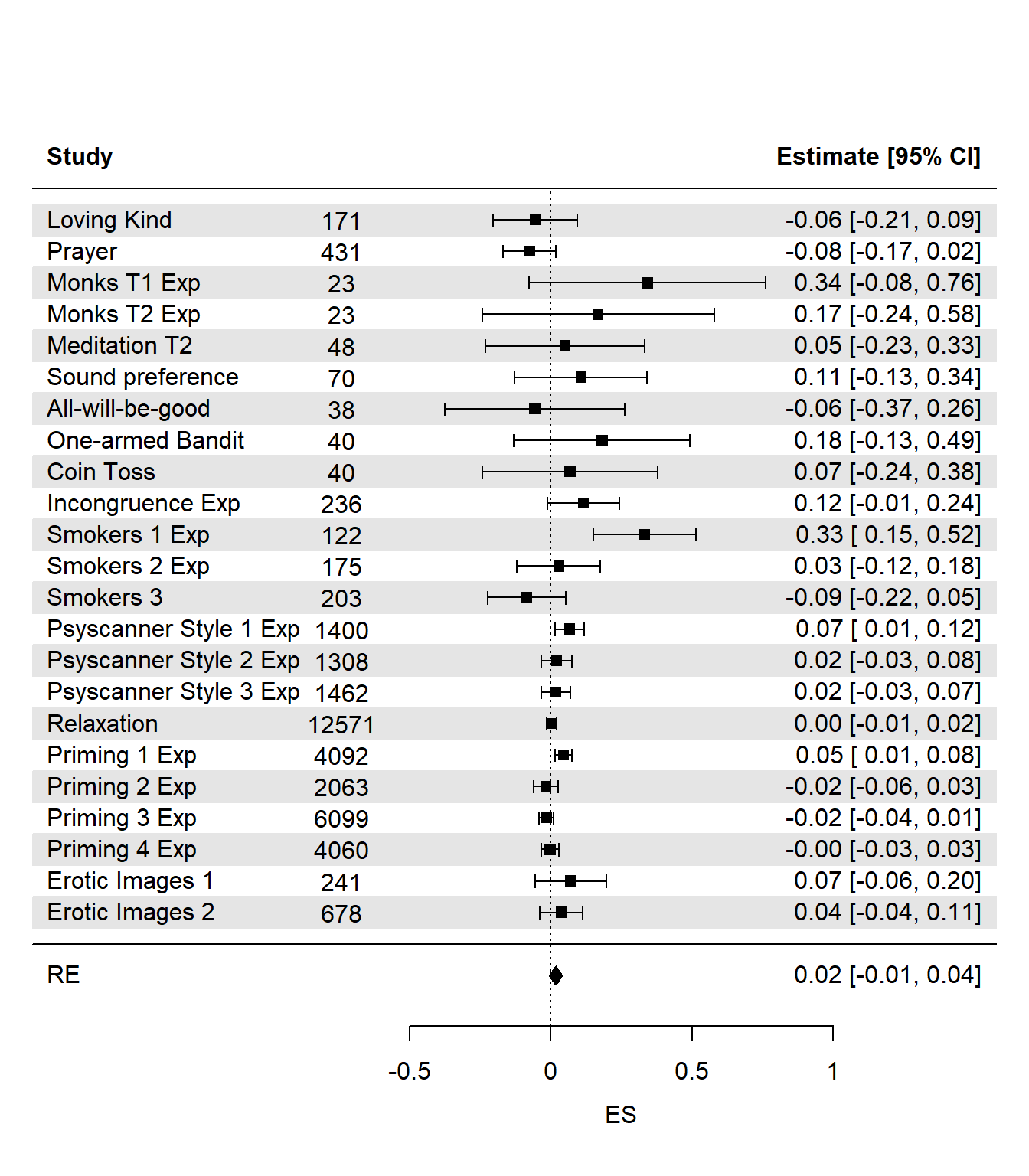
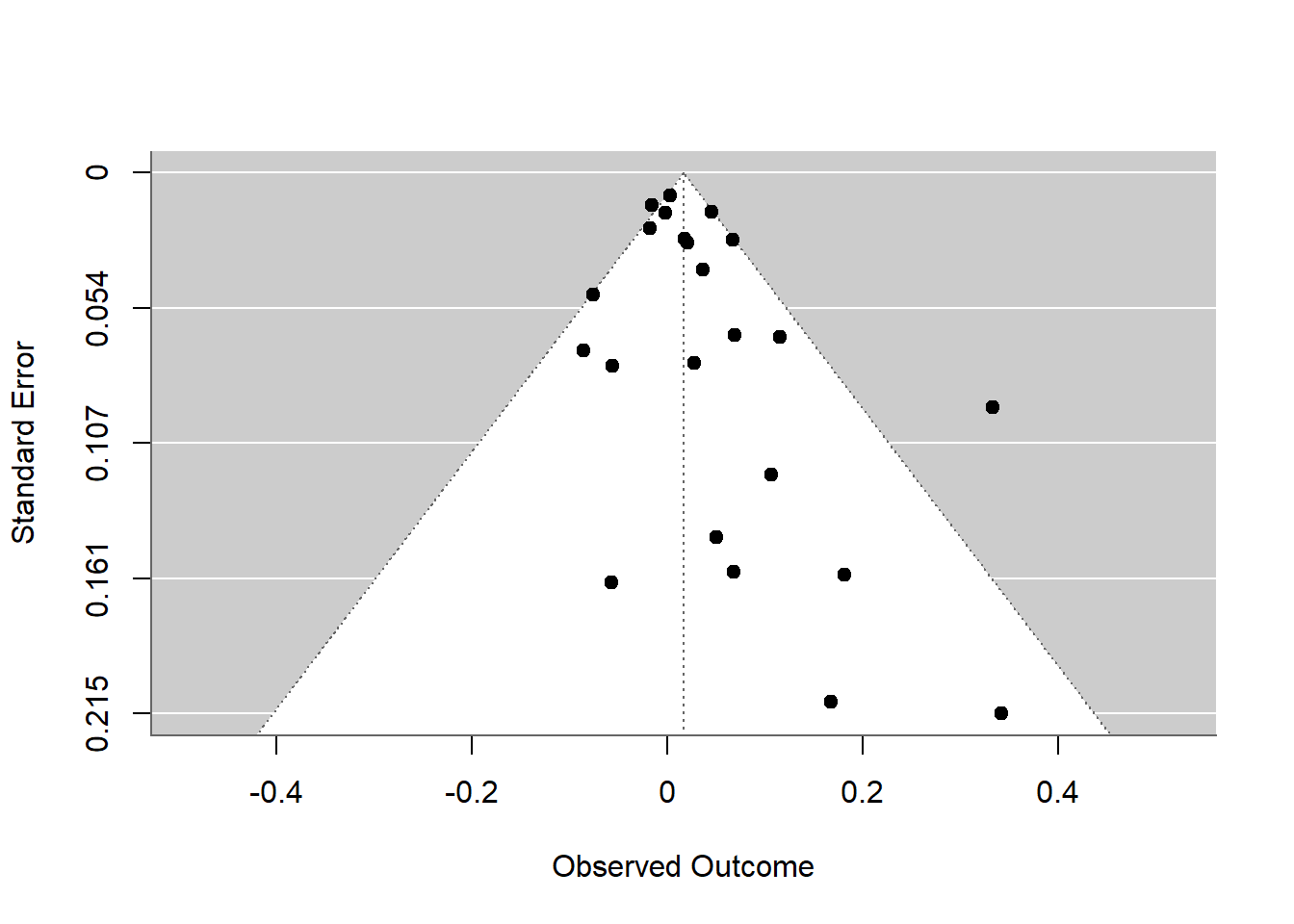
data <- subset(st, st$Experimental == TRUE)

knitr::kable(data)
Study Experimental N Trials M SD Hits (%) t p ES Var BF Direction Year Labstudy
1 Loving Kind TRUE 171 100 49.7251462 4.9301485 49.72515 -0.7290206 0.7665039 -0.0557496 0.0058570 0.3034712 greater 2016 TRUE
2 Prayer TRUE 431 100 49.6380510 4.8058917 49.63805 -1.5635507 0.9406706 -0.0753136 0.0023268 0.1448423 greater 2017 FALSE
3 Monks T1 Exp TRUE 23 400 202.3478261 6.8596892 50.58696 1.6414415 0.0574628 0.3422642 0.0460249 1.8155253 greater 2016 TRUE
5 Monks T2 Exp TRUE 23 400 201.3478261 8.0204777 50.33696 0.8059304 0.2144544 0.1680481 0.0440922 1.0456588 greater 2016 TRUE
8 Meditation T2 TRUE 48 100 50.2291667 4.5393766 50.22917 0.3497646 0.3640389 0.0504842 0.0208599 0.7452738 greater 2016 FALSE
9 Sound preference TRUE 70 40 20.3142857 2.9317990 50.78571 0.8968906 0.1864480 0.1071989 0.0143678 1.2000567 greater 2017 TRUE
10 All-will-be-good TRUE 38 100 49.7105263 5.0985313 49.71053 -0.3499901 0.6358347 -0.0567759 0.0263582 0.4729100 greater 2016 TRUE
11 One-armed Bandit TRUE 40 200 101.1250000 6.1818075 50.56250 1.1509781 0.1283746 0.1819856 0.0254140 1.2718689 greater 2017 TRUE
12 Coin Toss TRUE 40 200 100.5250000 7.7094265 50.26250 0.4306924 0.3345315 0.0680985 0.0250580 0.8018915 greater 2017 TRUE
13 Incongruence Exp TRUE 236 10 5.1822034 1.5779940 51.82203 1.7738101 0.0386948 0.1154652 0.0042655 2.2417309 greater 2017 FALSE
15 Smokers 1 Exp TRUE 122 400 196.7049180 9.8741574 50.82377 -3.6859216 0.0003423 -0.3337077 0.0086531 66.0635985 different 2015 TRUE
17 Smokers 2 Exp TRUE 175 400 200.2914286 10.3751851 49.92714 0.3715825 0.6446721 0.0280890 0.0057165 0.0902946 less 2016 TRUE
19 Smokers 3 TRUE 203 400 199.1379310 10.1117856 50.21552 -1.2146808 0.1129529 -0.0852539 0.0049440 0.3958797 less 2017 TRUE
20 Psyscanner Style 1 Exp TRUE 1400 30 15.1800000 2.6787278 50.60000 2.5142470 0.0060201 0.0671961 0.0007159 10.4147205 greater 2018 FALSE
22 Psyscanner Style 2 Exp TRUE 1308 30 15.0581040 2.7078599 50.19368 0.7760390 0.2189332 0.0214575 0.0007647 0.4976420 greater 2018 FALSE
24 Psyscanner Style 3 Exp TRUE 1462 30 15.0485636 2.7351180 50.16188 0.6789043 0.2486530 0.0177556 0.0006841 0.4146918 greater 2018 FALSE
26 Relaxation TRUE 12571 100 50.0177392 5.0616804 50.01774 0.3929391 0.3471856 0.0035046 0.0000795 0.0993029 greater 2016 FALSE
27 Priming 1 Exp TRUE 4092 20 10.1023949 2.2658819 50.51197 2.8907394 0.0019318 0.0451899 0.0002446 19.8004286 greater 2018 FALSE
29 Priming 2 Exp TRUE 2063 20 9.9612215 2.2326926 49.80611 -0.7888809 0.7848638 -0.0173685 0.0004848 0.0884220 greater 2018 FALSE
31 Priming 3 Exp TRUE 6099 20 9.9640925 2.3146664 49.82046 -1.2115083 0.8871262 -0.0155130 0.0001640 0.0364067 greater 2019 FALSE
33 Priming 4 Exp TRUE 4060 20 9.9955665 2.1896934 49.97783 -0.1290108 0.5513223 -0.0020247 0.0002463 0.0840137 greater 2020 FALSE
35 Erotic Images 1 TRUE 241 200 100.5103734 7.3155725 50.25519 1.0830494 0.1399367 0.0697653 0.0041595 0.9734614 greater 2017 FALSE
36 Erotic Images 2 TRUE 678 50 25.1283186 3.5249347 50.25664 0.9478799 0.1717644 0.0364031 0.0014759 0.6359922 greater 2017 FALSE
37 Smokers Priming Exp TRUE 38 20 10.0263158 1.9240560 50.13158 0.0843122 0.4666314 0.0136772 0.0263183 0.6764936 greater 2021 TRUE
44 Robots TRUE 34 10 5.2941176 1.6611316 52.94118 1.0324202 0.1546914 0.1770586 0.0298728 1.1772660 greater 2023 FALSE
45 Games TRUE 205 1-6 0.9121951 1.3365516 50.81522 0.1567684 0.4377912 0.0109492 0.0048783 0.4697811 greater 2023 FALSE
46 Schrödingers Cat Exp TRUE 285 10 4.8315789 1.5965586 48.31579 -1.7808771 0.9619993 -0.1054901 0.0035283 0.1605112 greater 2023 FALSE
47 Schrödingers Cat Con TRUE 285 10 5.0842105 1.5855631 50.84211 0.8966135 0.1853423 0.0531108 0.0035137 0.7779826 greater 2023 FALSE
48 Desire TRUE 201 10 5.0149254 1.5920980 50.14925 0.1329087 0.4471996 0.0093747 0.0049753 0.4651694 greater 2023 FALSE
49 Stories TRUE 766 1 0.5065274 0.5002841 50.65274 0.3611095 0.3590586 0.0130474 0.0013056 0.3452430 greater 2023 FALSE
50 Willpower TRUE 703 20 9.9843528 2.2960476 49.92176 -0.1806900 0.5716685 -0.0068149 0.0014225 0.2376857 greater 2023 FALSE
51 Baseline 1 Lucky TRUE 801 20 11.7990012 2.1279800 50.83749 -2.6732654 0.0038324 -0.0944552 0.0012540 10.8726734 less 2024 FALSE
52 Baseline 1 Unlucky TRUE 725 20 8.0000000 2.1784986 50.00000 0.0000000 0.5000000 0.0000000 0.0013793 0.2660541 greater 2024 FALSE
53 Baseline 2 TRUE 2094 20 12.0176695 2.1911024 49.92638 0.3690207 0.6439252 0.0080642 0.0004776 0.1286240 less 2024 FALSE

Forest Plot

The forest plot visually represents the effect sizes and confidence intervals for each study.

#Frequentist m-a with metafor 
library(metafor)

# Specify parameters of Exp Studies
yi=data$ES
vi=data$Var
studies=data$Study

# invert ES of Smokers 1, since the hypothesis was two-sided and the results showed a negative effect (smokers are avoiding smoking-related images)
yi[which(studies == "Smokers 1 Exp")] <- -yi[which(studies == "Smokers 1 Exp")]

# invert ES of studies with "less" hypothesis
yi[which(studies == "Smokers 2 Exp")] <- -yi[which(studies == "Smokers 2 Exp")]
yi[which(studies == "Smokers 3")] <- -yi[which(studies == "Smokers 3")]
yi[which(studies == "Baseline 1 Lucky")] <- -yi[which(studies == "Baseline 1 Lucky")]
yi[which(studies == "Baseline 2")] <- -yi[which(studies == "Baseline 2")]

# Recommended method = REML: Langan et al. 2018 https://onlinelibrary.wiley.com/doi/10.1002/jrsm.1316
# knha = Hartung method to control ES non-normality Rubio-Aparicio et al. 2018

res <- rma(
  yi,
  vi, 
  method="REML",
  #mods = ~ data$Labstudy,
  knha=TRUE,
  slab=paste(studies)
  )

# forest plot
forest(res, 
       xlab="ES", mlab="RE", psize=1,
       ilab = data$N, ilab.lab = "N",
       header=T, shade=T)

Summary Statistics

These are the results of the meta-analysis. The model results reflect the overall estimated effect size, its confidence interval and whether it differs significantly from 0.

The Tau² represents the between-study variance, and the I² the heterogeneity. A significant test for Heterogeneity indicates a genuine variability of true effects across studies.

summary.rma(res)

Random-Effects Model (k = 34; tau^2 estimator: REML)

  logLik  deviance       AIC       BIC      AICc   
 39.2253  -78.4505  -74.4505  -71.4575  -74.0505   

tau^2 (estimated amount of total heterogeneity): 0.0005 (SE = 0.0004)
tau (square root of estimated tau^2 value):      0.0231
I^2 (total heterogeneity / total variability):   36.71%
H^2 (total variability / sampling variability):  1.58

Test for Heterogeneity:
Q(df = 33) = 54.8958, p-val = 0.0097

Model Results:

estimate      se    tval  df    pval    ci.lb   ci.ub    
  0.0164  0.0088  1.8601  33  0.0718  -0.0015  0.0344  . 

---
Signif. codes:  0 '***' 0.001 '**' 0.01 '*' 0.05 '.' 0.1 ' ' 1

Funnel Plot

# funnel plot (publication bias)
funnel(res)

In this analysis all Micro-Pk studies of the LMU Micro-Pk Lab are included that hypothesize the absence of an effect. In studies comparing experimental to control conditions, only the control conditions are included. To ensure comparability, all studies are tested with directional hypotheses in the same direction as the corresponding experimental conditions.

# Select studies / conditions
data <- subset(st, st$Experimental == FALSE)

knitr::kable(data)
Study Experimental N Trials M SD Hits (%) t p ES Var BF Direction Year Labstudy
4 Monks T1 Con FALSE 29 400 198.344828 9.791672 49.58621 -0.9103017 0.8147832 -0.1690388 0.0349754 0.4860153 greater 2016 TRUE
6 Monks T2 Con FALSE 29 400 199.793103 9.648758 49.94828 -0.1154731 0.5455529 -0.0214428 0.0344907 0.6493717 greater 2016 TRUE
7 Meditation T1 FALSE 40 100 49.275000 5.764558 49.27500 -0.7954300 0.7844109 -0.1257685 0.0251977 0.4651069 greater 2016 FALSE
14 Incongruence Con FALSE 271 10 5.044280 1.538962 50.44280 0.4736623 0.3180617 0.0287729 0.0036916 0.5443204 greater 2017 FALSE
16 Smokers 1 Con FALSE 132 400 200.530303 9.682312 49.86742 0.6292627 0.5302729 0.0547703 0.0075871 0.1630540 different 2015 TRUE
18 Smokers 2 Con FALSE 220 400 198.981818 10.341636 50.25455 -1.4603179 0.0728179 -0.0984546 0.0045675 0.5477955 less 2016 TRUE
21 Psyscanner Style 1 Con FALSE 1003 30 15.061815 2.691409 50.20605 0.7273804 0.2335814 0.0229674 0.0009973 0.5395911 greater 2018 FALSE
23 Psyscanner Style 2 Con FALSE 1095 30 15.172603 2.740845 50.57534 2.0838687 0.0187019 0.0629743 0.0009151 4.3233628 greater 2018 FALSE
25 Psyscanner Style 3 Con FALSE 941 30 14.882040 2.637678 49.60680 -1.3718490 0.9147811 -0.0447210 0.0010638 0.1008342 greater 2018 FALSE
28 Priming 1 Con FALSE 4092 20 10.025660 2.260601 50.12830 0.7261019 0.2339089 0.0113509 0.0002444 0.2331401 greater 2018 FALSE
30 Priming 2 Con FALSE 2063 20 10.015511 2.234278 50.07756 0.3153284 0.3762721 0.0069425 0.0004847 0.2230455 greater 2018 FALSE
32 Priming 3 Con FALSE 6099 20 9.965076 2.362713 49.82538 -1.1543547 0.8758000 -0.0147812 0.0001640 0.0375426 greater 2019 FALSE
34 Priming 4 Con FALSE 4060 20 9.904926 2.255174 49.52463 -2.6862364 0.9963722 -0.0421581 0.0002465 0.0272478 greater 2020 FALSE
38 Smokers Priming Con FALSE 38 20 10.052632 2.459920 50.26316 0.1318916 0.4478923 0.0213956 0.0263218 0.6922438 greater 2021 TRUE
39 Sobjectivity 1 FALSE 898 20 9.989978 2.171804 49.94989 -0.1382877 0.5549780 -0.0046147 0.0011136 0.2204340 greater 2021 FALSE
40 Sobjectivity 2 FALSE 986 20 9.904665 2.261808 49.52333 -1.3235296 0.9070168 -0.0421498 0.0010151 0.1094664 greater 2021 FALSE
41 Sobjectivity 3 FALSE 1503 20 9.993347 2.221720 49.96673 -0.1160997 0.5462055 -0.0029947 0.0006653 0.1782954 greater 2023 FALSE
42 Epsi Correlation Condition A FALSE 2052 20 9.962476 2.259830 49.81238 -0.7521878 0.7739878 -0.0166050 0.0004874 0.1029726 greater 2021 FALSE
43 Epsi Correlation Condition B FALSE 2052 20 9.943470 2.255655 49.71735 -1.1352636 0.8718012 -0.0250616 0.0004875 0.0843100 greater 2021 FALSE

Forest Plot

The forest plot visually represents the effect sizes and confidence intervals for each study.

#Frequentist m-a with metafor 
library(metafor)

# Specify parameters of Exp Studies
yi=data$ES
vi=data$Var
studies=data$Study

# invert ES of studies with "less" hypothesis
yi[which(studies == "Smokers 2 Con")] <- -yi[which(studies == "Smokers 2 Con")]

# Recommended method = REML: Langan et al. 2018 https://onlinelibrary.wiley.com/doi/10.1002/jrsm.1316
# knha = Hartung method to control ES non-normality Rubio-Aparicio et al. 2018

res <- rma(
  yi,
  vi, 
  method="REML",
  #mods = ~ data$Labstudy,
  knha=TRUE,
  slab=paste(studies)
  )

# forest plot
forest(res, 
       xlab="ES", mlab="RE", psize=1,
       ilab = data$N, ilab.lab = "N",
       header=T, shade=T)

Summary Statistics

These are the results of the meta-analysis. The model results reflect the overall estimated effect size, its confidence interval and whether it differs significantly from 0.

The Tau² represents the between-study variance, and the I² the heterogeneity. A significant test for Heterogeneity indicates a genuine variability of true effects across studies.

summary.rma(res)

Random-Effects Model (k = 19; tau^2 estimator: REML)

  logLik  deviance       AIC       BIC      AICc   
 29.6427  -59.2854  -55.2854  -53.5047  -54.4854   

tau^2 (estimated amount of total heterogeneity): 0.0002 (SE = 0.0003)
tau (square root of estimated tau^2 value):      0.0149
I^2 (total heterogeneity / total variability):   23.10%
H^2 (total variability / sampling variability):  1.30

Test for Heterogeneity:
Q(df = 18) = 21.3290, p-val = 0.2631

Model Results:

estimate      se     tval  df    pval    ci.lb   ci.ub    
 -0.0076  0.0072  -1.0481  18  0.3084  -0.0228  0.0076    

---
Signif. codes:  0 '***' 0.001 '**' 0.01 '*' 0.05 '.' 0.1 ' ' 1

Funnel Plot

# funnel plot (publication bias)
funnel(res)

Change of Evidence
 

© 2024-2025 Dr. Moritz Dechamps